Hermite Spline
These are my recent study notes on splines, specifically on Hermite Splines. The knowledge mainly comes from Wikipedia and the background knowledge comes from GAMES102.
The frequently used Hermite Spline generally refers to Cubic Hermite Spline, and it belongs to the same category of cubic polynomial splines as Bézier curves.
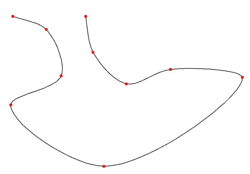
Cubic polynomial splines generate interpolation curves within small ranges between two control points, and the integration of these curves forms the whole interpolation curve.
The interpolation curve generated by the Hermite spline is continuous and passes through all control points. Each control point needs to comprise information about the position vector and the tangent vector. However, in practical applications, we often only attain determined position vector information, whereas the tangent vector needs to be estimated by further setting up logic.
Interpolation Formula
Assume that the interpolation range of $t$ is $t\in [0,1]$.
The position and tangent of the starting point and the ending point are respectively denoted as $\overrightarrow{p}_k, \overrightarrow{m}_k, \overrightarrow{p}_{k+1}, \overrightarrow{m}_{k+1}$.
Here, the subscript of the starting point is $k$.
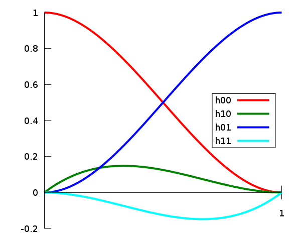
$$ \begin{aligned} \overrightarrow{p}(t)&=h_{00}(t)\overrightarrow{p}_k+h_{10}(t)\overrightarrow{m}_k+h_{01}(t)\overrightarrow{p}_{k+1}+h_{11}(t)\overrightarrow{m}_{k+1},\\ h_{00}(t)&=2t^3-3t^2+1,\\ h_{10}(t)&=t^3-2t^2+t,\\ h_{01}(t)&=-2t^3+3t^2,\\ h_{11}(t)&=t^3-t^2. \end{aligned} $$
The interpolation parameters of other ranges just need to be proportionally resized to $[0,1]$.

$h_{00}(t),h_{01}(t),h_{10}(t),h_{11}(t)$ are referred to as Hermite basis functions. They can also be expressed in the form of a linear combination of Bernstein bases.
| expanded | factorized | Bernstein | |
|---|---|---|---|
| $h_{00}(t)$ | $2t^3-3t^2+1$ | $(1+2t)(1-t)^2$ | $B_0(t)+B_1(t)$ |
| $h_{10}(t)$ | $t^3-2t^2+t$ | $t(1-t)^2$ | $\cfrac13B_1(t)$ |
| $h_{01}(t)$ | $-2t^3+3t^2$ | $t^2(3-2t)$ | $B_3(t)+B_2(t)$ |
| $h_{11}(t)$ | $t^3-t^2$ | $t^2(t-1)$ | $-\cfrac13B_2(t)$ |
Positions and tangents can be represented as coefficients to express this cubic polynomial in its standard form.
$$ \overrightarrow{p}(t)=(2\overrightarrow{p}_k+\overrightarrow{m}_k-2\overrightarrow{p}_{k+1}+\overrightarrow{m}_{k+1})t^3+(-3\overrightarrow{p}_k+3\overrightarrow{p}_{k+1}-2\overrightarrow{m}_k-\overrightarrow{m}_{k+1})t^2+\overrightarrow{m}_kt+\overrightarrow{p}_k. $$
This format is more efficient for multiple calculations where control points remain the same while the value of t changes, as coefficients can be calculated once and reused.
Estimating Tangents from Control Point Positions
A reasonable estimation of tangents is crucial to guarantee the continuity of the entire curve at each connecting point formed by sections of curves. Moreover, it should achieve $C_2$ continuity, ensuring that the curve is smooth.
There are many methods for estimating tangents, with several common ones recorded in Wikipedia.
Sometimes, the value of $t$ does not fall within $[0,1]$, but falls within any interpolation interval of arbitrary length between two control points, denoted as $t\in[x_{k+1},x_k]$. The length between two control points is $x_{k+1}-x_k$. When different values are taken for $k$, $x_{k+1}-x_k$ might also be different. If they are all the same, it’s referred to as uniform parameter spacing.
Finite difference
$$ \overrightarrow{m}_k=\cfrac12(\cfrac{\overrightarrow{p}_{k+1}-\overrightarrow{p}_k}{x_{k+1}-x_k}+\cfrac{\overrightarrow{p}_{k}-\overrightarrow{p}_{k-1}}{x_{k}-x_{k-1}}). $$
The finite difference does not require the parameter spacing to be uniform.

Cardinal spline
$$ \overrightarrow{m}_k=(1-c)\cfrac{\overrightarrow{p}_{k+1}-\overrightarrow{p}_{k-1}}{x_{k+1}-x_{k-1}} $$
Where $c\in[0,1]$, is referred to as the tension parameter. In some sense, it can be interpreted as the “length” of the tangent. Selecting $c = 1$ results in all tangents having length 0, while selecting $c = 0$ results in the Catmull-Rom spline under uniform parameterization. It is said that changing $c$ can manipulate the shape of the curve, making it closer or farther from the control points.

Catmull–Rom spline
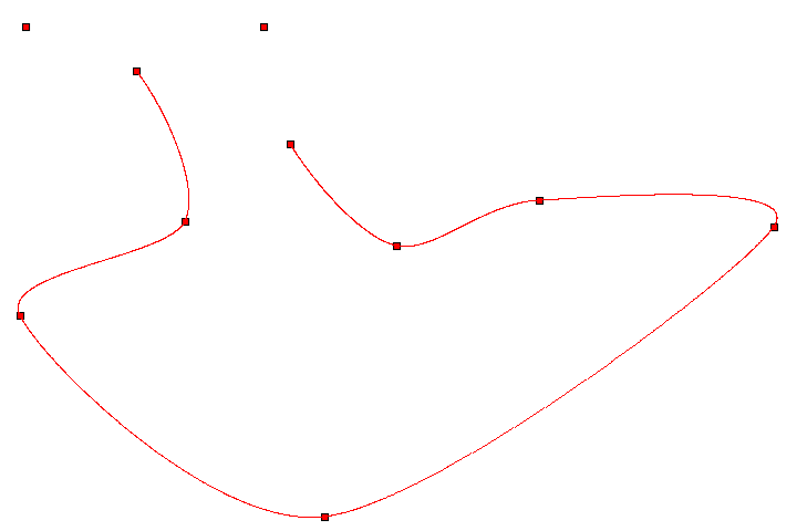
It is a particular case of the cardinal spline that I use the most. This simple formula requires the parameter spacing to be consistent.
$$ \overrightarrow{m}_k=\cfrac{\overrightarrow{p}_{k+1}-\overrightarrow{p}_{k-1}}2 $$
Curves implemented this way can form a cyclic path. The Catmull-Rom spline is often used to achieve smooth interpolated motion between keyframes. The main reason for its popularity is it’s relatively easy to calculate, ensures accurate hits on each keyframe position, and guarantees continuity of the generated curve’s tangent across multiple sections.
